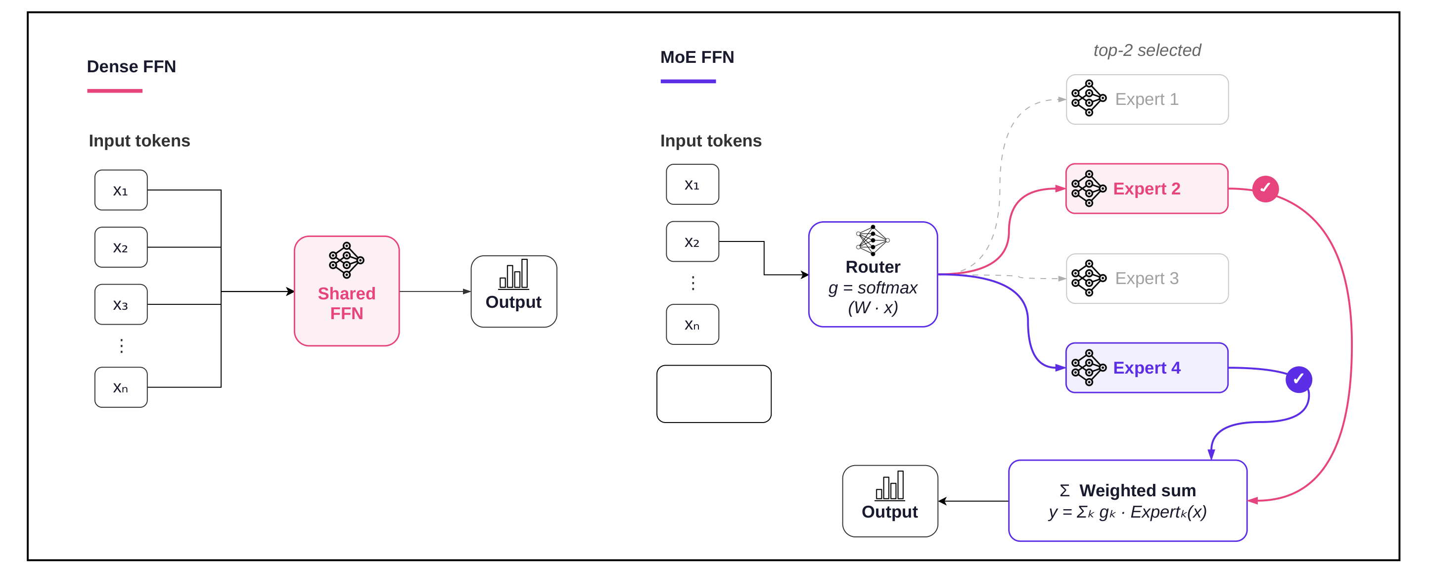
Mixture-of-Experts (MoE) models carry far more parameters than they activate. For each token that passes through, a learned router selects only a small subset of specialized sub-networks called experts to run, leaving the rest idle. The result is a model that scales in capacity without scaling proportionally in per-token compute.
This post walks through how that works in two parts. The first explains the architecture from the ground up: how the router makes decisions, how the system stays balanced, and how specialization emerges through training rather than design. The second reports what actually happened when we tried to fine-tune a 35-billion-parameter multimodal MoE on four A100 GPUs, including five sharding approaches that all failed, what finally worked, and what a layer-by-layer routing audit revealed about how the model allocates capacity across audio, video, and text. A runnable notebook covering the full training pipeline is linked at the end.
Most modern language models are built on the Transformer architecture[1], which has made it practical to train large sequence models efficiently at scale. These models process text as tokens: small units such as words, word fragments, or punctuation. Since then, progress has largely followed a clear pattern. When model size, training data, and compute are scaled together, performance tends to improve[2].
Dense scaling has a direct cost: every token uses the same full feed-forward capacity at each layer. In dense models, adding feed-forward capacity therefore increases not only the total model size, but also the computation, memory, energy, and serving infrastructure required to train and serve the model. This raises a practical question: can we give a model more capacity without making every token pay for all of it?
Mixture-of-Experts (MoE) is a neural network architecture that decomposes a model into multiple specialized sub-networks, called experts, and dynamically routes inputs to the most relevant experts for a given task. Originally proposed in early work on modular neural networks, MoE adopts a divide-and-conquer strategy in which computation is distributed across multiple specialized experts[3][4]. Unlike dense models that activate all parameters for every input, MoE models use a router to selectively activate only the most relevant experts, increasing capacity while maintaining computational efficiency.
MoE also offers a different scaling strategy: to increase total model capacity without activating all of it for every token. Rather than expanding one shared feed-forward network (FFN), an MoE layer typically replaces it with a collection of expert FFNs and a learned router[5]. For each token, the router selects a small subset of experts to run, while the remaining routed experts stay inactive. This is known as conditional computation.
For example, an MoE layer may contain 16 experts but route each token to only the top two. Across tokens, the model can draw from the full pool of 16 experts, while any given token activates only two. This is the central MoE trade-off: more total parameters, but only a subset of expert parameters activated per token. Switch Transformers[6], a simplified MoE architecture, show that sparse routing scales to extremely large models while keeping the routing mechanism simple, including a top-1 configuration in which each token is sent to a single expert.
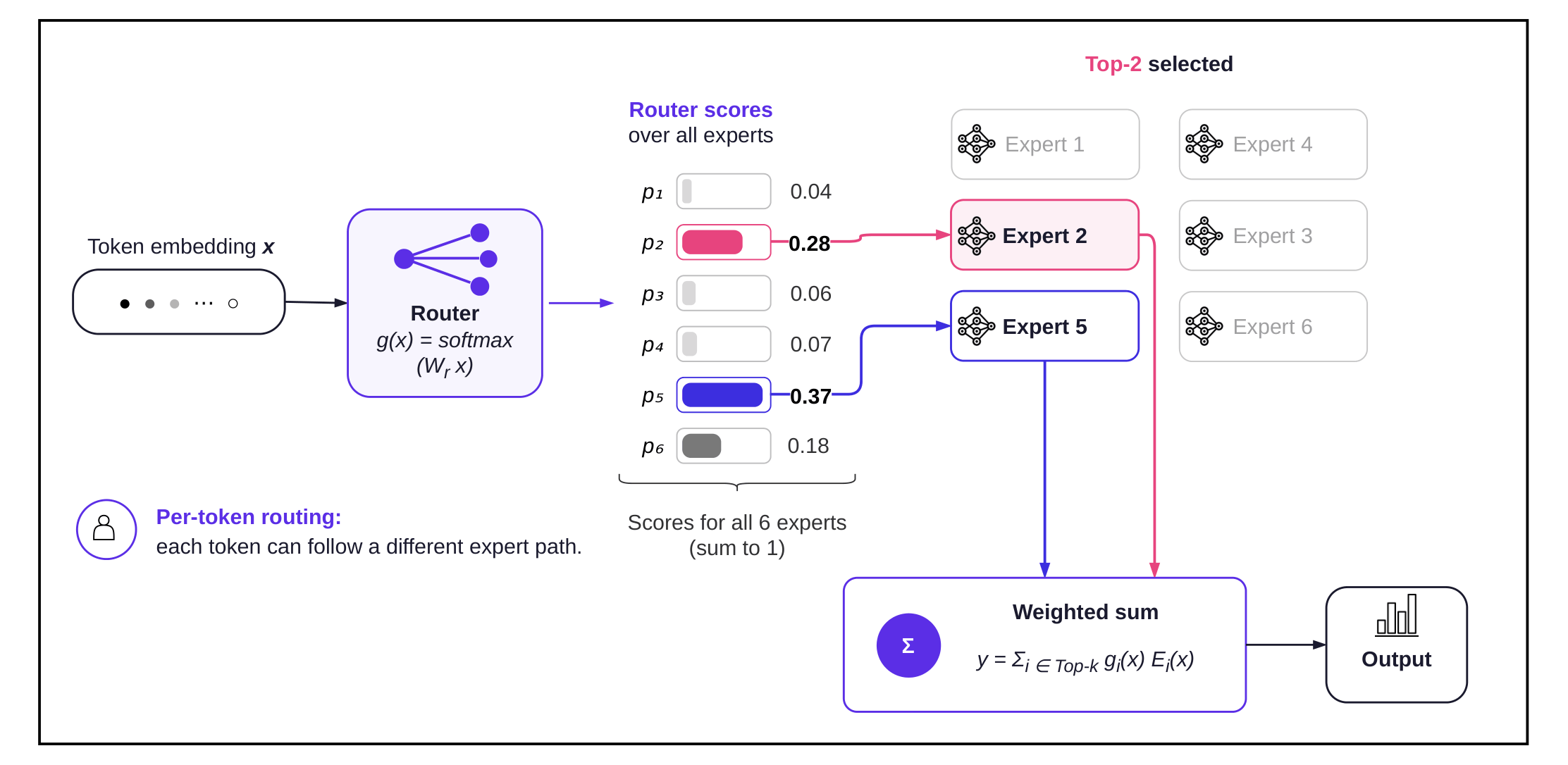
The router decides which experts process each token, which is what makes MoE conditional. For each token representation \(x\), the router produces one score for every available expert:
where \(W_r\) is a learned routing matrix. These scores are normalized with a softmax to form a probability distribution over experts:
The model then selects the top-\(k\) experts with the highest routing probabilities. If \(k = 2\), the token is dispatched to its two most relevant experts; if \(k = 1\), it is sent to only one. The final output is a weighted combination of the selected expert outputs:
In Eq. \eqref{eq:moe-output} the gate values come directly from the full softmax; many recent MoE models (for example Mixtral[7] and DeepSeek[8]) instead renormalize the gates over the selected top-\(k\) so that the combination weights post selection sum to one. The motivation is that the full softmax distributes probability mass across all \(E\) experts, so the top-\(k\) gates may sum to well below one, particularly when the router's distribution is flat. Without renormalization, a token routed through an uncertain, broadly spread distribution would produce a low-magnitude output simply because most of the probability mass fell on experts that were not selected. Renormalizing after selection restores the output scale and ensures that the relative weighting among the chosen experts reflects the router's preference among them, rather than being diluted by probability assigned to unchosen experts. Both variants are common. Importantly, the router makes this decision per token and at each MoE layer. Two tokens from the same sentence can therefore follow different expert paths, and the same word can be routed differently depending on its context and representation at a given layer.
Because MoE modifies the architecture rather than the training objective, it can be applied to any task that a dense Transformer supports, including generation, classification, translation, and multimodal reasoning. Routing allows an MoE model to use capacity selectively. It also introduces a new challenge: without constraints, the router can repeatedly send too many tokens to the same few experts, leaving others underused. We address that next through load balancing and expert-capacity controls.
The router's purpose is to reduce per-token compute by selecting only the most relevant experts. But this creates a tension. Left unconstrained, the router learns to concentrate tokens on a small number of experts that perform well early in training, starving the rest of useful gradients and reinforcing the imbalance. The result is expert collapse: a model with 128 experts that effectively uses only a handful of them, negating the capacity advantage that motivated the MoE design. The problem is compounded in distributed settings, where experts are spread across devices and one overloaded expert can stall an entire layer[9].
Load-balancing mechanisms address this by encouraging the router to spread tokens more evenly. This comes at a cost: pushing tokens toward underutilized experts means some tokens are processed by experts that are not their best match. The balancing objective and the routing objective are therefore in direct competition. Too little balancing leads to expert collapse; too much flattens the routing distribution and erodes the specialization that makes MoE useful. The methods below represent different points along this trade-off.
A common solution is a load-balancing loss. Let \(f_i\) be the fraction of tokens sent to expert \(i\) and \(P_i\) the average routing probability for that expert. Switch Transformers[6] use
where \(E\) is the number of experts and \(\alpha\) controls how strongly the model is encouraged to spread work across them. Minimizing this product penalizes configurations where an expert both receives a large share of tokens and carries high average routing probability, pushing the router toward more uniform assignment.
Each expert also has a limited number of tokens it can process in one batch. For \(T\) tokens, top-\(k\) routing, and \(E\) experts, this limit is often written as
where \(c\) is the capacity factor. If an expert receives more tokens than its limit, extra assignments may be dropped or sent through another routing path[10][6].
Other methods balance experts more directly. BASE Layers frame assignment as a balanced optimal-transport problem[11], Expert Choice Routing lets each expert select a fixed number of tokens[5], and newer approaches adjust routing biases without an auxiliary loss[12]. At extreme sparsity ratios, Kimi K3 takes this further with Quantile Balancing, which derives expert allocation directly from router-score quantiles, removing the balancing hyperparameter \(\alpha\) entirely[13].
Balanced traffic is only the first step toward specialization. Experts can receive comparable numbers of tokens while still learning redundant or overly broad functions[14]. This problem can be addressed at three levels: architecture, training objectives, and post-hoc analysis.
DeepSeekMoE[15] replaces a small pool of large experts with a larger pool of finer-grained experts, activating more of these smaller components per token while keeping the compute budget similar. It also separates shared experts, which run for every token and capture broadly useful language patterns, from conditionally selected routed experts, which can focus on information specific to the current token and context.
Architecture is not the only lever. Guo et al.[14] show that conventional balancing objectives can still encourage overly uniform routing and overlapping experts, and they introduce objectives intended to make expert selection more discriminative while retaining balanced utilization.
Specialization can be measured rather than assumed. Olson et al.[16] find that routing decisions change when the same word appears in different semantic contexts, suggesting that some expert choices reflect contextual meaning rather than surface token identity.
These three perspectives converge on a common point: experts are not predefined modules such as “the code expert” or “the reasoning expert.” Their roles develop from expert granularity, routing policy, training objectives, and data. This becomes especially important in multimodal models, where routing must allocate capacity across text, images, audio, and their interactions.
This section assumes some familiarity with distributed training frameworks. If you have worked with DeepSpeed[8] or PyTorch Fully Sharded Data Parallel (FSDP)† before, you will recognize the tools; the failure modes described here are specific to MoE layers and are not documented in most practical guides.
Standard distributed-training tools shard parameters across devices and gather them on demand during the forward pass. We tested five such configurations across two frameworks on a 35.26B-parameter multimodal MoE model and all five failed. The root cause is architectural: data-dependent routing means the framework cannot know which expert weights are needed until routing has already occurred, making the gather-on-demand model fundamentally incompatible with sparse MoE layers. This section documents those failures, explains why expert parallelism is the correct long-term alternative, and describes the memory-reduction pipeline that made fine-tuning feasible within project constraints.
This section uses Qwen3-Omni-30B-A3B[17], a multimodal MoE model built on Qwen's Thinker–Talker architecture, as a working case. The full checkpoint has 35.26B parameters; the “30B” in the name refers to the Thinker. The fine-tuning target is a structured multimodal output task.
Large dense models are often trained with parameter sharding: the weights of each layer are partitioned across devices, and during the forward pass each device temporarily gathers the full layer weights it needs, runs the computation, and releases them. DeepSpeed ZeRO-3[18] and PyTorch FSDP[19] follow this pattern. It works well for dense Transformers because the same layers process every token, so the sequence of gather, compute, and release operations is identical for every input in the batch.
MoE layers break that assumption. Routing is data-dependent: different tokens in the same batch may select different experts at runtime. A sharding framework that partitions layer weights cannot know in advance which expert weights will be needed, because that decision depends on the router output, which itself depends on the forward pass reaching that layer. In practice, this forces the framework to gather many or all experts before routing can proceed, pushing peak memory back toward the unsharded model size and erasing the benefit of sharding.
This is the core problem: parameter sharding distributes weights across devices by layer, but in an MoE model the relevant unit of distribution is the expert, not the layer. Section 6.3 describes why expert parallelism, which distributes by expert rather than by layer, is the natural fit.
We tested five sharding configurations across two frameworks on a 35.26B MoE model with 48 layers and 128 experts per layer, targeting four 80 GB A100 GPUs. All configurations failed.
FULL_SHARD. Wrapping the native MoE decoder layers forced FSDP to gather all 128 experts before routing could proceed, reproducing the full model footprint on each device. Peak allocation was 77.99 GiB.NotImplementedError: Cannot copy out of meta tensor; no data!), exposing an incompatibility between HuggingFace's from_pretrained (which builds a skeleton on a meta device) and DeepSpeed's _post_init method (which attempts to copy data to the local device immediately).uint8 with a separate quant-state metadata object. The partitioning logic splits the raw uint8 storage but discards the quant state, making the reconstructed parameters meaningless on each rank.SHARD_GRAD_OP. A partial-sharding variant that retains full parameters during the forward pass. Peak allocation was 77.99 GiB, equivalent to the full model size.The consistency of this failure across two frameworks and five configurations confirms that the root cause is architectural rather than a tuning issue: data-dependent routing is fundamentally incompatible with the gather-on-demand model of parameter sharding.
| Configuration | Framework | Failure mode | Peak memory |
|---|---|---|---|
| ZeRO-2 (bf16) | DeepSpeed | OOM on activation alloc | 78.56 GiB |
FSDP FULL_SHARD | PyTorch | Full expert gather | 77.99 GiB |
| ZeRO-3 (bf16) | DeepSpeed | Meta-tensor crash | — |
| ZeRO-3 + QLoRA | DeepSpeed | Optimizer crash | — |
FSDP SHARD_GRAD_OP | PyTorch | Full model size retained | 77.99 GiB |
Expert Parallelism (EP) avoids this problem by distributing experts rather than layer weights. Each device permanently owns a disjoint subset of experts, and tokens are dispatched to whichever device holds their selected experts via all-to-all communication. No reassembly is required.
Feasibility tests confirmed that a single MoE layer and a full 48-layer forward pass both ran without errors under DeepSpeed EP. However, EP could not be used for fine-tuning from a pretrained checkpoint. DeepSpeed's MOELayer class is architecturally distinct from the HuggingFace MoE implementation: it registers experts under its own internal naming convention (nn.ModuleList) rather than the pretrained model's mlp.experts layout. Loading pretrained weights into DeepSpeed EP structure would require a multi-gigabyte weight remapping pipeline and a custom forward-pass patch to reconcile incompatible return signatures. This made EP non-viable for fine-tuning within project constraints. We flag it as the appropriate long-term direction for large-scale MoE training.
Rather than shard expert weights across devices, the working setup kept each MoE layer intact and placed complete layers on individual devices using device_map="auto". This allowed routing to happen locally within each layer, avoiding cross-device expert gathering during the forward pass.
This addressed the failure mode above: standard sharding struggled because expert weights had to be reconstructed around data-dependent routing. Keeping layers intact removed that issue but made memory the main constraint.
Because device_map="auto" balances by parameter count rather than layer count, the vision encoder (543M parameters) and audio encoder (600M parameters) added extra load to early devices, leaving them with fewer Thinker layers. In practice, this imbalance did not create visible stalls. The final setup depended on three memory reductions, summarized in Table 2. Removing any one of them caused an out-of-memory failure.
| Optimization | Implementation | Peak memory |
|---|---|---|
| Baseline | Full 35.26B model, bf16 | 70.5 GB |
| QLoRA (4-bit) | NF4 frozen weights; LoRA adapters in bf16 | 17.85 GB |
| Flash Attention 2 | Tiled attention; \(O(N)\) vs. \(O(N^2)\) memory | OOM prevented† |
lm_head pre-hook | Hidden states sliced to \(\sim\)350 positions | 15.6 GB |
†Flash Attention 2 does not lower the short-sequence peak; it removes the \(O(N^2)\) attention-matrix allocation that would otherwise OOM at long sequence length. Its effect is visible only at large frame counts.
QLoRA quantized the frozen base weights to 4-bit NF4[20], while LoRA adapters[21] remained trainable in bf16. This reduced the largest fixed memory cost without updating the full 35.26B parameters.
Flash Attention 2[22] addressed the long-sequence bottleneck. At the largest evaluated input, standard attention would materialize an \(N \times N\) attention matrix per layer; tiled attention avoids that allocation while preserving the same output.
lm_head pre-hook.The final projection was another major bottleneck because it would produce logits for all token positions over a 152,000-entry vocabulary. Since only about 350 answer-position tokens contributed to the loss, a forward hook sliced the hidden states before the projection, reducing logit memory from 23.3 GB to 0.3 GB.
This pipeline was stress-tested at 128 frames (28,746 tokens), reaching a peak of 60.06 GB and remaining within the same hardware envelope at the largest evaluated input size.
Section 6 showed how to make a multimodal MoE model trainable. Before fine-tuning it, we needed to understand what the router had already learned. This section audits the routing structure across all 48 layers of the Thinker. For multimodal models the relevant question is whether the router treats audio, visual, and text tokens as distinct computational problems, or whether it routes all modalities through a common set of experts. We ran a routing analysis across all 48 MoE layers on 13 distinct video topic domains, capturing expert-activation patterns per modality and per layer.
To measure routing consistency across topics, we computed the Jaccard similarity of activated expert sets for the same modality across topic domains. A similarity of 1.0 would mean the model routes identical expert sets regardless of what the token represents semantically. A lower value indicates topic-sensitive routing.
Across the first 28 layers, average Jaccard similarity held at 0.9731, indicating that early routing is nearly identical regardless of topic content. Across the full 48 layers, global similarity dropped to 0.8804.
This reveals a structural transition. In layers 1–28, the router assigns tokens to experts based primarily on modality: audio tokens follow audio pathways, visual tokens follow visual pathways, and the assignment is stable regardless of what is being said or shown. In layers 29–48, routing begins to differentiate by semantic content. The same audio token representing speech in one topic domain is sent to meaningfully different experts than the same audio token in another domain, even within the same modality class. Routing in the deeper layers reflects what the token means in context, not just what kind of signal it is.
To measure how consistently each modality uses the same experts across the early and late halves of the network, we extracted the top-20 activated experts per modality in layers 1–28 and layers 29–48 and measured their overlap.
| Modality | Expert overlap (top 20) | Stability |
|---|---|---|
| Audio | 18 / 20 | High |
| Video | 16 / 20 | Moderate |
| Text | 11 / 20 | Low / dynamic |
Audio and video tokens maintain consistent expert pathways across the full depth of the network: the experts that process perceptual signals in early layers continue to handle them in deep layers. Text tokens show substantially greater routing volatility. Fewer than half of the top-20 text experts are shared between the shallow and deep layers, indicating that the model dynamically reassigns text to different experts as it moves from perceptual encoding toward higher-level reasoning.
This pattern matches what we would expect from a model trained on diverse multimodal data: perceptual processing is handled by stable, specialized pathways, while language-level reasoning draws on a more flexible, context-dependent set of experts.
This asymmetry has practical consequences for fine-tuning: adapting text routing may require more capacity or longer training than adapting audio or video routing, because the text pathways are less stable and more sensitive to distributional shift between pretraining and fine-tuning data.
Gating entropy measures how concentrated or distributed routing decisions are at each layer. High entropy means tokens are spread broadly across experts; low entropy means a small number of experts dominate. Values below are in nats; with 128 experts the theoretical maximum is \(\ln 128 \approx 4.85\).
Entropy peaked at 3.97 in layer 5, indicating distributed, exploratory routing in early layers. It then declined monotonically after that peak to a minimum of 3.12 by layer 47. This decay confirms progressive specialization: as tokens approach the output, routing becomes increasingly concentrated, and the model commits to a narrow set of highly relevant experts before producing its final representation.
Importantly, the audit found no permanently dead experts. While isolated layers contained small inactive pools, every one of the 128 experts was activated at least once across the 48-layer, 13-topic evaluation. The router uses the full expert capacity of the model.
The routing structure observed before fine-tuning was already well organized, by modality in early layers and by semantic content in later layers. This raised the question of whether fine-tuning the router would improve task performance or risk disrupting a stable, useful structure.
Because the routing tables were already deeply converged and the full expert pool was actively utilized, we froze the MoE router (all mlp.gate parameters) for fine-tuning. This had two consequences. First, it eliminated the need for an auxiliary load-balancing loss \(\mathcal{L}_{\text{bal}}\) (Eq. \eqref{eq:balance}), which is typically required to prevent expert collapse when routing is trainable[6]. Since expert utilization was already balanced, the penalty was unnecessary, and removing it simplified the training objective. Second, it concentrated the entire trainable-parameter budget on the Thinker's dense attention projections (q_proj, k_proj, v_proj, o_proj), preserving the routing structure the model had already developed while adapting how it attends to multimodal inputs.
Fine-tuning large MoE models from pretrained checkpoints raises several open questions that the experiments above surface but do not fully resolve.
EP is theoretically the correct distributed strategy for sparse models: it avoids the data-dependent gather problem by co-locating each expert on a dedicated device. Current framework implementations, however, are designed for training from random initialization and assume ownership of the expert architecture. Using EP for fine-tuning from a pretrained HuggingFace checkpoint requires reconciling incompatible expert-registration formats and return signatures. Closing this gap would make EP practical for fine-tuning and is an important direction for frameworks that aim to support sparse-model adaptation.
Our findings suggest that routing structure is already meaningful before task-specific fine-tuning. It is not yet clear how robust this structure is under longer training runs, larger learning rates, or distribution shift between pretraining and fine-tuning data. Methods for monitoring routing stability during fine-tuning, analogous to gradient-norm tracking for dense models, would be a useful practical contribution.
For multimodal sequences, the number of tokens per example is a function of both modality count and temporal resolution. Our experiments show diminishing returns from uniform frame sampling: increasing from 16 to 64 frames improved validation loss by 0.079, while a further increase to 96 frames gained only 0.029 at 1.5 times the compute. This suggests that a token-selection strategy, deciding which frames and audio segments to include rather than sampling uniformly, may yield greater improvements than simply increasing sequence length.
Fine-tuning an MoE model on structured-output tasks introduces a period during which the model's general output format is partially disrupted before the task-specific format is learned. In our experiments, roughly 20% of one-epoch evaluation entries produced no valid output at all, not because the model lacked the relevant knowledge, but because it had not yet stabilized the expected response structure. Standard accuracy metrics do not distinguish between format failures and reasoning failures. Evaluation protocols that account for this distinction would give a more informative picture of task-specific learning progress during early training.
The full QLoRA training pipeline, including the 4-bit NF4 setup, Flash Attention 2 configuration, and lm_head pre-hook, is available as a runnable notebook:
The notebook walks through every step shown in Section 6 and Section 6.4 on a single SONIC-O1 sample entry. Model weights and the full 13-topic routing evaluation set are not released due to size and licensing constraints.
† PyTorch FSDP tutorial: https://docs.pytorch.org/tutorials/intermediate/FSDP_tutorial.html ↩